To Use Overhead or Underground Transmission? That is (Still) the Question (Part II)

Download the full pdf of this article, which includes the inline equations and diagrams.

Discussion continues at the national level about power grid upgrades to support increased electrification. In fact, since the first part of this article series ran (T&D World March 2022), Pacific Gas & Electric Co. publicized more details on its plans to put 3600 miles (5794 km) of distribution lines in California underground over the next half decade, with the goal of scaling up toward that number and topping 1000 miles (1609 km) annually in both 2025 and 2026. The utility is talking with seven firms about its overall plan to bury 10,000 miles (16,093 km) of distribution lines as part of a plan to help the California power grid operate more safely and resiliently. Plans such as this highlight the importance of careful characterization of underground cable limits.

The first part of this article series discussed the specific issues utilities need to consider when evaluating the use of alternating-current (ac) high-voltage cables for long-distance transfer of electrical power. The high costs of design and construction, shorter asset life and maintenance challenges of high-voltage cable systems should be considered by utilities and grid operators when weighing underground vs. overhead options for transmitting bulk electrical power.

In this second part, the focus turns to the ac cable length limitations imposed by electrical impedance characteristics. It is generally understood that ac cable lengths are constrained by their capacitive current. A simple calculation of cable current rating divided by charging current per length often is used to estimate maximum allowable cable length. However, further examination of transmission line impedance characteristics leads to a more general approach for estimating maximum cable length. This article discusses these concepts at a high level, and links are provided at the end to an online calculator and more detailed technical information. Application of these concepts can assist utilities in assessing and planning for increased deployment of underground T&D facilities.

The Optimal State

It is important to review transmission line basics pertinent to this discussion. For simplicity, examples are discussed on a per-phase basis. While helpful for illustrative purposes, actual three-phase equations that include mutual coupling should be used for analysis.

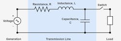
The first figure in this article illustrates a simple transmission line connected between a source and a load. The line is modeled with a shunt capacitance and a series resistance and inductance. A variant of this model (not shown) places half the capacitance on either side of the inductance and resistance. This model is valid for lengths less than about 100 km (62 miles). If the load is disconnected from the energized line by opening the switch, current can still flow in the loop that remains through the resistor, inductor and capacitor. The impedance of the capacitor dominates and the current into the line is approximately proportional to the total capacitance, which in turn is proportional to the length of the line. The current in this no-load case is sometimes referred to as a charging current. Because the current is dominated by the capacitance, reactive power is exported by the line and must be absorbed by the source.

A 345-kV underground cable system (199-kV line to ground) has a charging current on the order of 10 A to 20 A per km. Therefore, an energized open-circuited 10-km (6.2-mile) length of cable may have between 100 A to 200 A of charging current. Beyond some length, the capacitive current alone will exceed the thermal limit, which is on the order 800 A to 1500 A per phase for a typical transmission cable.

This simple method of using charging current to identify maximum length cannot be applied generally to all transmission lines. As an example, consider the case of overhead transmission lines, which have about one-tenth the capacitance of underground lines (that is, one-tenth of the charging current). If no-load charging current limits the length of high-voltage cable to values on the order of tens of km, then universal application of the simplified method would mean high-voltage overhead lines could not exceed lengths on the order of hundreds of km. However, operational experience indicates no such limit applies to overhead line lengths.

In the case of overhead lines, the simplified method fails because it does not account for the inductive properties of the circuit. The reactive power consumed because of current flow in the inductor is subtracted from the overall reactive power supplied by the capacitance. The result is a reduction in the amount of reactive power the generator needs to absorb and a corresponding reduction of the total input current to the line.

To explore this further, assume the switch in the first figure is closed to connect a resistive load to the line. The voltage drop across the relatively small series resistance and inductance is negligible. Therefore, the voltage across the capacitance does not change much and reactive power supplied by the capacitance  is approximately constant despite changing load. However, as load current increases, the reactive power consumed by the series inductance increases significantly (, where v is the frequency in radians per sec.).

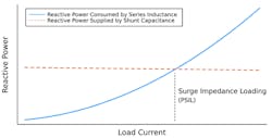
The following figure shows a plot of inductor and capacitor reactive power as functions of load current. At some point the load current is such that reactive power consumed by the inductance is the same as reactive power supplied by the capacitance. No reactive power is supplied to the line or absorbed from the line by external generation. This is called the surge impedance loading . The load resistance that gives this load level is called the surge, or characteristic, impedance and is calculated as  . Surge impedance loading can be calculated as  .

Topology And SIL Differences

Two different topologies are used for transmission lines in these examples as shown in the middle figure on page 43. The first is a closed topology of two coaxial conductors separated by a dielectric material that fills the space between them. This topology is used for most underground cables. The second is an open topology of two parallel cylindrical conductors separated by some distance in free space. Configurations like this (or with additional wires) historically have been used for overhead transmission lines.

The closed topology of power cables gives characteristic impedances on the order of 20 ohms to 60 ohms (high capacitance and low inductance). The open topology of overhead transmission lines gives characteristic impedances on the order of 200 ohms to 400 ohms (low capacitance and high inductance). Hence, the surge, or characteristic, impedance of an open wire transmission system is on the order of 10 times larger than that of a coaxial cable.

All high-voltage power lines have thermal limits on how much power they can transfer safely. For overhead lines, these limits have their origin in the maximum temperatures of conductors, derived using the type of conductor as well as a balance between ohmic/solar heating and cooling due to convection (wind) and thermal radiation. If thermal limits are violated, excess conductor sagging and loss of conductor strength may occur. For underground lines, heat sources include ohmic losses, dielectric loss and magnetic losses, if enclosed in steel pipe. Heat dissipation is constrained by the thermal conductivity and temperature of the materials in which the line is embedded. If cable thermal limits are violated, more rapid deterioration of insulating material occurs. This shortens the life of the cable. Generally, thermal limits for underground lines are more severe; they must be operated at lower temperatures and, consequently, cannot carry as much current as overhead lines for the same voltage class and conductor diameter. As an example, the per-phase surge impedance loading for a 345-kV overhead transmission line (199-kV line to ground) with a typical 250-ohm surge impedance is 159 MW (about 800 A per phase). This is reasonable for an overhead line and consistent with many years of experience.

By contrast, an underground transmission line designed for the same voltage will have a much smaller surge impedance, generally around 40 ohms. In this case, the surge impedance loading becomes about 5000 A (about 992 MW). This is much larger than thermal limits typically allow for any single underground cable. Consequently, safe operation of the cable would be well below the surge impedance loading and still results in export of reactive power, even sometimes for
relatively short lines. The bottom line is the reduced surge impedance coupled with reduced thermal limits of underground lines results in an ac length limit that is difficult to overcome.

Finding Length Limits

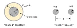
It is primarily the difference in voltage angle that drives real power flow from one bus to the other.

Further, it is possible to derive an expression in which the magnitude of complex power is shown as some fraction of the surge impedance loading. Equation 1 is conceptual, but shows that the normalized complex power magnitude has real power and reactive power components that are each functions of both line length and voltage phase angle difference. In detailed form, the equation would include parameters associated with wave characteristics and dielectric material properties:
              (Eq. 1)

where P1 and Q 1 are the sending end of real and reactive components of the complex power. At the surge impedance loading, there is no reactive power, and the real power can be written as follows:
                (Eq. 2)

Both real and reactive power contribute to the current at the input to the line. Hence, for conditions in which Eq. 1 is greater than Eq. 2, the real power transmitted will be less because excess reactive power of the cable (which counts against thermal limits) is exported to the rest of the power system.
To determine line length limits, the constant contour values of Eq. 1 and Eq. 2 can be plotted as functions of both ∆θ and line length. More specifically, the constant values represent specific rated power flow as a fraction of the surge impedance loading. Different underground transmission lines will have thermal limits that are different percentages of their respective surge impedance loading.

Contour plots of the total complex power magnitude (that is, Eq. 1) in red and real power (that is, Eq. 2) in dashed black are plotted in the graph on the next page. One well-known characteristic of cables easily can be discerned from this graph. For zero real power transferred (that is, phase angle difference equal to zero), the maximum allowed complex power magnitude at the line input (in this case, all reactive power) increases linearly as the line length increases. This is consistent with the idea that capacitive current is larger for longer line lengths when there is no real power transfer (for example, no load and no voltage difference between the generators).

Once the fraction of rated cable current to surge impedance loading is determined, the thermally safe operating conditions for the cable are enclosed by the region to the left of the corresponding contour. For example, if the cable thermal rating is 20% of the surge impedance limit, the only portion of the plot that corresponds to allowable operation is to the left of the 20% contour in the graph (solid red contour lines).

It is important to note that even the no-load case (that is,  assumes sources are connected to both ends of the cable and each absorbs the same amount of reactive power. If a cable is unloaded but energized from only one end, the theoretical maximum line length would be about half that indicated in the figure. In such a situation, it also is important to consider the steady-state voltage at the open end of the cable.

Some Examples

In this section, maximum line lengths are determined using a single-phase representation of commercially available 1500-kcmil cross-linked polyethylene (XLPE) cable designed for several different voltages. The hard length limit is determined by finding the maximum length for the no-load case (that is, . The practical length limit is the longest length for which the total power and real power are approximately equal. Lengths longer than the stated practical length limit could be used but would have to be derated for real power transfer. Again, it should be emphasized the limits derived here are for lines between voltage buses with equal voltage amplitude (that is, the same reactive power is exported at each end of the cable). Limits for other situations may be smaller. (See Table 1) It is clear from the table the practical use of underground cable is limited to lengths less than the theoretical hard limit. Further, the higher the voltage, the shorter the practical length limit.

Maximizing Length

Options for mitigating line length constraints are few. A cooling system could be used to raise the thermal limits of underground lines. However, this would require additional infrastructure and add substantially to the cost of underground transmission lines. Reactive compensation distributed at intermediate points along the line could be used to reduce that portion of the cable ampacity used up by reactive power flow. This could be done using shunt reactors, although the amount of compensation needed would depend on the load required. Furthermore, using shunt reactors could cause other operational issues, such as unintended resonances. High-voltage shunt reactors are costly, often require a small substation and present switching challenges that require special-purpose circuit breakers designed to interrupt inductive currents.

High-voltage direct-current (HVDC) could be used since there is no reactive power at dc. Note also the length of any transmission line as a fraction of wavelength becomes zero in this case. In fact, HVDC transmission lines are used exclusively for long undersea connections for which no ac system would be possible. However, dc transmission lines require both special cable and costly ac-dc converter terminals at each end.

Fundamental Differences

Fundamental differences exist between underground and high-voltage ac transmission lines because of their topology and heat-transfer characteristics. For underground lines, these differences result in length limits that are more restrictive for higher voltages. The same limits do not apply to overhead lines because they can be operated at or near surge impedance loading. As a result, replacing long ac overhead with long ac underground high-voltage transmission lines presents
major challenges derivable from fundamental physics.

The approach discussed in this article for determining maximum ac cable length is general and can provide insight into hard and practical length limits. The analysis suggests that, from a physics perspective, maximizing power flow for a given underground cable length is not necessarily achieved with the maximum voltage, as is often the case with overhead lines.

For More Information

Those who want to learn more about the theory behind this article can consult a background paper at www.electricutilitytools.com/education/ugtransmission. A free calculator also is available at www.electricutilitytools.com/calculators. This calculator allows estimation of maximum theoretical and practical ac cable lengths using detailed three-phase-based computation.

Download the full pdf of this article, which includes the inline equations and diagrams.

Robert G. Olsen ([email protected]) is professor emeritus in the School of Electrical Engineering and Computer Science at Washington State University. He received his Ph.D. and MSEE degrees from the University of Colorado Boulder in 1970 and 1974, respectively, and his BSEE degree from Rutgers University in 1968. He has been with Washington State University since 1973. His other positions included senior scientist with the Westinghouse Georesearch Laboratory in Colorado; NSF faculty fellow with GTE Laboratories in Massachusetts; a visiting scientist with ABB corporate research in Sweden and the Electric Power Research Institute (EPRI) in California; and a visiting professor with the Technical University of Denmark. His work has been featured in approximately 250 refereed journals and conferences. He is one of the authors of the EPRI AC Transmission Line Reference Book — 200 kV and Above (EPRI, 2005). Olsen is an honorary life member of the IEEE Electromagnetic Compatibility (EMC) Society. He also is a past U.S. National Committee representative of CIGRE Study Committee 36 (EMC) and a past chair of IEEE Power & Energy Society ac fields and corona effects working groups. In addition, he is a past associate editor for the IEEE Transactions on Electromagnetic Compatibility and Radio Science.

Jon T. Leman ([email protected]), P.E., is a principal engineer with the consulting firm POWER Engineers, Inc. where he specializes in AC and DC overhead and underground transmission line electrical design. He also is co-owner of the software company Electric Utility Design Tools LLC. Leman earned his Ph.D. degree in electrical and computer engineering from Washington State University in 2021 and his MSEE and BSEE degrees from the University of Idaho in 2010 and 2001, respectively. He taught courses in physics and electrical engineering for the U.S. Navy from 2001 to 2005. In 2005, he joined POWER Engineers. His technical interests are electromagnetics, power system transients, equipment failure investigation, numerical methods, insulation coordination, and power system planning. The focus of his doctoral research was application of electromagnetics to optimize high-voltage transmission line design. He is a member of CIGRE and a senior member of IEEE.